Bits, Bits, Bits

This post is one of my white whales – the problem that has eluded me for far too long and drove me to the edge of insanity.  I’m talking about writing binary.  Now, let me be clear when I say that I am far from a computer scientist: I don’t think in base 16, I don’t dream in assembly code, I don’t limit my outcomes to zeros and ones.  I do, however, digest material before writing about it, seek creative and efficient solutions to problems, and do my best to share this information with others (that’s where you come in).
​
First, let’s create a fake dataset with help from Nick Cox’s egenmore ssc command:

set obs 300
forvalues i = 1/200 {
        gen x`i' = round(runiform()*50*_n)
}

gen id = _n
reshape long x, i(id) j(vars)
egen count = xtile(x), nq(30)
keep id vars count

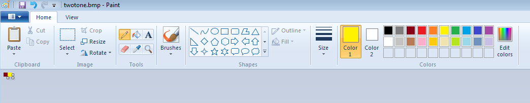
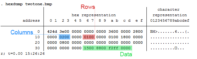
​​Today we will be making a bitmap of a map for Fitbit activities by writing bits of binned colors in a binary file.  Alliteration aside, this post pulls from various sources and is intended to cover a great deal of topics that might be foreign to the average Stata user – in other words, hold on tight!  It’s going to be a bumpy bitmap ride as we cover three major topics: (1) Color Theory, (2) Bitmap Structures, and (3) Writing Binary Files using Stata.

Color Theory​

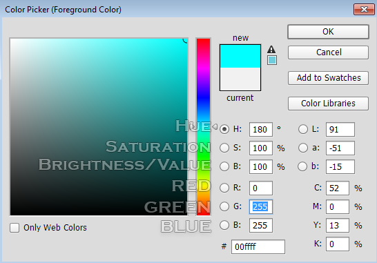
​In creating gradients, it was recommended to me to use a Hue, Saturation, Value (HSV) linear interpolation rather than the Red, Green, Blue (RGB) interpolation because it looks more “natural.”  I will not argue this point, as I know nothing about it.  For me, I know that if I play with the sliders in Photoshop, it automatically changes the numbers and I never have to think about what it’s actually doing in the conversion. In order to convert from RGB to HSV and vice versa, I used the equations provided here – to learn about what’s going on, Wikipedia has a great article on the HSV cones!

​Bitmap Structures

Uncompressed bitmaps are fairly easy to understand once you get the hang of them – they’re even easier to reverse engineer.  In MS Paint, simply create a two pixel 24-bit bitmap and save the resulting picture.  It’s a work of art, I know.  

From here, run a hexdump on the file in Stata (see below image).
​
For simplicity’s sake, the only things we'll need to change are the numbers of rows and columns in the bitmap header.

As for the body, there are three rules we need to keep in mind here:

1. The picture starts in the lower left-hand corner, reading right to left.  If you forget to do this, your picture will be vertically flipped.
2. The bytes are written in the opposite order for colors: instead of writing in RGB, you need to write in BGR.
3. All “columns” need to be divisible by four.  You need to add zeros as a buffer until your column is divisible by four.

The final step is to make sure that the rows and columns are written in correct order.  I did not find an efficient way to do this step, so input is always appreciated.  We can see that the box labeled “Columns” is pretty straight forward when it’s a small number under 256 pixels.  What happens when it exceeds 256 pixels?  We have to write it in reverse order!  For example: we will use Mata’s inbase() command to convert a theoretical picture's width of 500 pixels to base 16.  The result?

. mata: inbase(16, 500)
  1f4

​Let’s add a zero in front of that to get 01f4 as our width.  Once again, we must reverse this order; therefore, our real values to write are f4 and 01.  Converting these values using frombase() yields 244 and 1 respectively.  These are the bytes we’ll end up writing in the next section.

Writing Binary

First, please visit Phil Ender’s website on writing and reading binary data as it heavily influenced this sections, and also because Phil is a great guy.
​
My code broke out this task in two sections: writing the header and writing the body:

The Header
The header is fairly straight forward: just copy and paste the hexdump from before (converting from base 16 to base 10) or by reading in the file byte by byte.

file open myfile using testgrad.bmp, write replace binary
file write myfile %1b (66) %1b (77) %1b (70) %1b (0) %1b (0) %1b (0)
file write myfile %1b (0) %1b (0) %1b (0) %1b (0) %1b (54)
file write myfile %1b (0) %1b (0) %1b (0) %1b (40)
file write myfile %1b (0) %1b (0) %1b (0)

mata: bitmap_rowcol(bitmap_size(200), bitmap_size(300))
file write myfile %1bu (`c1') %1bu (`c2') %1bu (0) %1bu (0)
file write myfile %1bu (`r1') %1bu (`r2') %1bu (0) %1bu (0)

file write myfile %1b (1) %1b (0) %1b (24) 
file write myfile %1b (0) %1b (0) %1b (0) %1b (0) %1b (0) %1b (16)
forvalues i = 1/19 {
        file write myfile %1b (0)
}

​​Notice the order of the column and row variables.  I create these values using the separate function bitmap_rowcol() to deal with the problem mentioned earlier.  Think of `c1’ as 244 and `c2’ as 1, and `r1’ as 2c and `r2’ as 1 for a width of 500 pixels and a height of 300 pixels with rules according to our previous analysis.

The Body
From there, we call bitmap_body in mata and close our file (cols is 200 in my example)::

mata: bitmap_body(${cols}, X, buff)
file close myfile

​​This is all great, but I’m not going to lie, it means absolutely nothing to me without seeing the final result.  So here it is:

HSV Gradient with a 5 px Gaussian Blur

RGB Gradient with a 5 px Gaussian Blur

​This can now produce textures for our Fitbit elevation map in the next series quickly, and effectively, all within Stata.  The entire file is available here for those who are willing to put up with some messy code:

bitmap.do
File Size:	4 kb
File Type:	do

Download File

---