Category: Base16

HMAC-SHA1 in Stata

2/10/2016

Why Care Block?
Security and the Twitter API – You need this if you want Twitter to work with Stata

I applaud all of you who have made it this far, but unfortunately things are going to get super boring! Well, besides applause I’d also like to take a sentence to thank you for reading this content: whether you’re reading this out of boredom, coercion, to make fun of it, or you just have a general interest, I’d like to extend my gratitude.

Switching back to the good stuff, today we’re talking about hash functions. Think hash browns *delicious* - they’re sliced, diced, and fried to a golden brown; drenched or drizzled with hot sauce or ketchup (I prefer Cholula and Tabasco) and resembles nothing like the raw potato it once was. Now, take your hash browns and try to reconstruct the original potato. “No!” you’d say, “That’s really hard.” Keep in mind this post is about security, from a non-cryptographic scientist or security expert, so anticipate a lot more potato metaphors because that’s about all I know about security.

This post is really about making the Twitter API work within Stata without any outside plugins or packages. To do so, we must find a way to recreate the HMAC-SHA1 algorithm which is quite difficult without our previous toolset we designed, so make sure you’ve gone over the bitwise operators. Once we’re on the same page, we can start getting into this hash function in order to send requests using Twitter’s API so that you can retrieve you beautiful, crispy hash brown data in return.

The Fuss

HMAC-SHA1 is the type of procedure we’re trying to reproduce from the Wikipedia article available here. I didn’t care much for it. It didn’t explain what it is, what it was really doing, or why we should care at a simple level so that someone less savvy (like me) could understand just what the fuss is all about. Both HMAC and SHA1 are procedures. HMAC stands for Hash Message Authentication Code and is the procedure we use to combine a message with a secret key whereas SHA-1 stands for Security Hash Algorithm 1, which was made by the NSA and is used to break a message into a corresponding hash string with a fixed block size. Together, they make sure that the integrity of the data hasn’t been compromised and that you’re not sending your raw secret message over the internet…series of tubes. The nice thing about the SHA-1 algorithm is that very slight changes, say replacing a single character in the message, dramatically changes the resulting hash so that it’s difficult to crack (though apparently not secure enough for today’s standards). Remember, HMAC is the main procedure to combine a secret key with the message and SHA-1 is just the type of hash function implemented; but you probably don’t care that much and just want to see the code. So let’s get started!

The SHA-1

SHA-1 has a lot of destructive procedures, a lot of breaking bits into smaller bits, and a lot of the previously developed bitwise functions. Let’s see a quick example of this in action.
Say I have the string phrase "The Ore-Ida brand is a syllabic abbreviation of Oregon and Idaho" and I want to run the SHA-1 Function on it.

mata: sha1("The Ore-Ida brand is a syllabic abbreviation of Oregon and Idaho") 
The results is (hex): 156a5e19b6301e43794afc5e5aff0584e25bfbe7
In Base64: FWpeGbYwHkN5SvxeWv8FhOJb++c=

Good luck figuring out the original string from the Base64 encoding. Now remember, this is not a post about theory or reasoning behind the SHA-1 procedure; this post is about making it work. Therefore, the advanced Stata user who wishes to replicate/improve this code might find this next section interesting. Here are some of my observations regarding repackaging the SHA-1 function.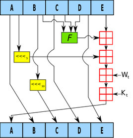

Mata is incredibly fast, but much slower than the C-code equivalent due to all bits being interpreted as strings and converted back to bytes.
All bytes are subject to integer overflow – if adding two base 2 integers exceeds 2^32, the number acts as an odometer, reverting to zero before counting up again.
While the Wikipedia makes a lot of reference to the “big-endian” integer, the resulting link has a lot of information we might not care about. For our purposes, “big-endian” means that it has left-padded zeros.
Say we needed the number 55 to be “big-endian” 16-bits. Well, 55 is 110111 in base 2 and, since this is only 6 numbers, we’d need it to have 10 preceding zeros.
If your integer padded message length final message is greater than 512 bits, you need to break it out into as many 512-bit sections as necessary to only have 512-bit chunks.
Initialize your “h” variables once (this should be a given). Each time we feed a block through our chunk-making process, overflow-add the “h” variables to the previous values until you run out of blocks.

The HMAC

Compared to SHA-1, the HMAC procedure is a walk in the potato fields… it’s easy as potatoes… I’m running out of references here. Did you know that the potato was the first vegetable to be grown in space? If astronauts could do that with potatoes, we can certainly make HMAC-SHA1 work with Stata. There’s really just a three step process at play. The HMAC procedure takes two inputs: a key and a message.

If the key is longer than the blocksize (64 in this case) run the SHA-1 function on the key; if it’s shorter, left pad the key with 0x00 (- char(0) -); if it’s the same length, just keep the key.
Create the outer key pad (64 * “\”) and the inner key pad (64 * “6”), convert these to their base 2 representation, and use the exclusive or bitwise operator on the key pad and the key.
Concatenate the inner key pad with your message (inner key pad first) and run the SHA-1 function on the resulting padded message. Take the outer key pad and concatenate the result of your first SHA-1 with the outer key pad (outer key pad first) and run the SHA-1 function on this step. Now we’re technically done!

The Conclusion

Well, this post (and the previous one) has been filled with a little more technical jargon than I planned. I like to keep these posts fun and poignant, but this material is for the dedicated and serves as a reference for those who want to expand Stata’s capabilities (even if it takes a little longer than expected). This new Mata function allows Stata to perform the HMAC-SHA1 procedure which is vital for enabling Twitter requests through Stata so that the entire process can be contained within one do-file. Here’s an example of the function in action:

. mata: hmac_sha1("Secret Key", "Message to be sent")
  d5052c13e868ea7c932be9279752e9e67c8195bd
. mata: hmac_sha1("Secret Key", "Message to be Sent")
  f67f5f90132583de85abf0d61fed2a2144be1f04

You can see how the examples show that slight changes in the message dramatically change the output. Feel free to download the process below. All subroutines are included for your convenience. Good luck!

hmac-sha1.do
File Size:	6 kb
File Type:	do

Download File

5 Comments

Just One More Binary Thing (I Promise)

10/26/2015

1 Comment

On writing binary files in Stata/Mata

As a supplement to my most recent posts, I decided to put together a quick guide on writing and reading binary files. Stata has a great manual for this – however, I struggled to see how this works in Mata. I spent a good afternoon scouring Google, Stata Journals, and Statalist to no avail. Little did I know, I was looking in the wrong places and for the wrong commands. It wasn’t until I broke out my old Mata 12 Mata Reference guide that I realized the solutions lie not with fopen(), but with bufio() (and yes, bufio() is referenced in fopen() - always check your references)

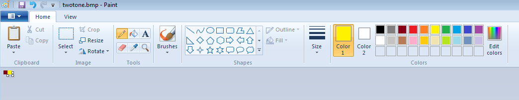
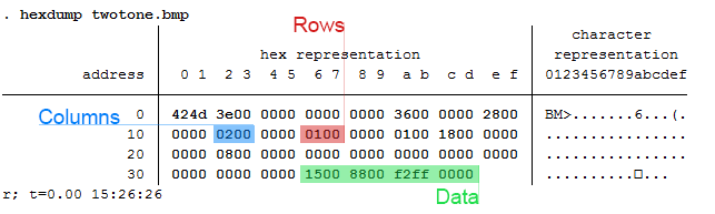
We start by making up a fake type of file called a wmm file. This file always begins with the hex representation ff00, which we know just means 255-0 in decimal or 11111111 00000000 in binary. The next 20 characters spell out “Will M Matsuoka File” followed by a single byte containing the byte order or 00000001 in binary. From there, the next four bytes contains the location of our data as we put a huge buffer of zeros before any meaningful data. It makes sense to skip all of these zeros if we know we don’t need to ever use them. After these zeros, we’ll store the value of pi and end the files with ffff.

The file looks like this:

Stata's File Command

tempname fh

file open `fh' using testfile.wmm, replace write binary

file write `fh' %1bu (255) %1bu (0)
file write `fh' %20s "Will M Matsuoka File"

file set `fh' byteorder 1
file write `fh' %1bu (1)

* offset 200
file write `fh' %4bu (200)

forvalues i = 1/200 {
        file write `fh' %1bs (0)
}

file write `fh' %8z (c(pi))
file write `fh' %2bu (255) %2bu (255)

file close `fh'

The only thing I feel I need to note here is the binary option under file open. Other than that, take note that we’re setting the byteorder to 1. This is a good solution to writing binary files; however, since most of my functions are in Mata, we might as well figure out how to do this in Mata as well.

Mata's File Command

If you didn’t know, Mata’s fopen() command is very similar to Stata’s file commands, with a few slight differences that we won't touch on here. Just know, it's pretty awesome and don't forget the mata: command!

mata:
fh = fopen("testfile-fwrite.wmm", "w")

fwrite(fh, char((255, 0)))
fwrite(fh, "Will M Matsuoka File")

// We know that the byte order must be 1
fwrite(fh, char(1))

fwrite(fh, char(0)+char(0)+char(0)+char(200))
fwrite(fh, char(0)*200)

fwrite(fh, char(64) + char(9) + char(33) + char(251) + 
        char(84) + char(68) + char(45) + char(24))

fwrite(fh, char((0,255))*2)
fclose(fh)
end

I personally like the aesthetic of this syntax; it’s clean, neat, and relatively simple. The only problem is its ability to handle bytes. In short, it doesn’t do it at all. We’d have to build some more functions in order to accomplish this task (especially when it comes to storing double floating points) which is why Mata also has a full suite of buffered I/O commands. It’s a little more complicated, but well worth it. After all, we cheated in converting pi to a double floating storage point by using what we wrote in the previous command. This is not a good practice.

Mata's Buffered I/O Command

Let's get right to it

mata:
fh = fopen("testfile3-bufio.wmm", "w")

C = bufio()
bufbyteorder(C, 1)

fbufput(C, fh, "%1bu", (255, 0))
fbufput(C, fh, "%20s", "Will M Matsuoka File")

// We know that the byte order must be 1
fbufput(C, fh, "%1bu", bufbyteorder(C))

fbufput(C, fh, "%4bu", 200)
fbufput(C, fh, "%1bu", J(1, 200, 0))

fbufput(C, fh, "%8z", pi())

fbufput(C, fh, "%2bu", (255, 255))
fclose(fh)
end

The one distinction here is the use of the bufio() function. It creates a column vector containing the information of the byte order and Stata’s version, but allows us to use a range of binary formats available to use in Stata’s file write commands.

Reading the Files Back

Now that we’ve written three files, which (in theory) should be identical, let’s create a Mata function that reads the contents stored in these files. Note: it should return the value of pi in all three cases. As it turns out, they all do.

mata:
void read_wmm(string scalar filename)
{
        fh = fopen(filename, "r")
        C = bufio()

        fbufget(C, fh, "%1bu", 2)
        if (fbufget(C, fh, "%20s")!="Will M Matsuoka File") {
                errprintf("Not a proper wmm file")
                fclose(fh)
                exit(610)
        }
        
        bufbyteorder(C, fbufget(C, fh, "%1bu"))

        offset = fbufget(C, fh, "%4bu")
        fseek(fh, offset, 0)

        fbufget(C, fh, "%8z")

        fclose(fh)
}

read_wmm("testfile-fwrite.wmm")
read_wmm("testfile.wmm")
read_wmm("testfile3-bufio.wmm")
end

And there you have it, a bunch of different ways to do the same thing. While I enjoy using Mata’s file handling commands for its simplicity, it does get a little cumbersome when writing integers longer than 1 byte at a time. Time to start making your own secret file formats and mining data from others.

1 Comment

Bits, Bits, Bits

10/5/2015

1 Comment

This post is one of my white whales – the problem that has eluded me for far too long and drove me to the edge of insanity. I’m talking about writing binary. Now, let me be clear when I say that I am far from a computer scientist: I don’t think in base 16, I don’t dream in assembly code, I don’t limit my outcomes to zeros and ones. I do, however, digest material before writing about it, seek creative and efficient solutions to problems, and do my best to share this information with others (that’s where you come in).

First, let’s create a fake dataset with help from Nick Cox’s egenmore ssc command:

set obs 300
forvalues i = 1/200 {
        gen x`i' = round(runiform()*50*_n)
}

gen id = _n
reshape long x, i(id) j(vars)
egen count = xtile(x), nq(30)
keep id vars count

Today we will be making a bitmap of a map for Fitbit activities by writing bits of binned colors in a binary file. Alliteration aside, this post pulls from various sources and is intended to cover a great deal of topics that might be foreign to the average Stata user – in other words, hold on tight! It’s going to be a bumpy bitmap ride as we cover three major topics: (1) Color Theory, (2) Bitmap Structures, and (3) Writing Binary Files using Stata.

Color Theory

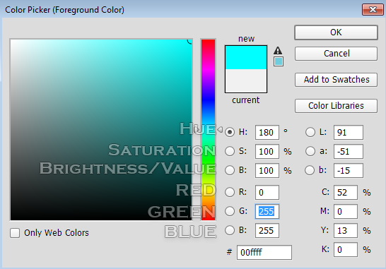
In creating gradients, it was recommended to me to use a Hue, Saturation, Value (HSV) linear interpolation rather than the Red, Green, Blue (RGB) interpolation because it looks more “natural.” I will not argue this point, as I know nothing about it. For me, I know that if I play with the sliders in Photoshop, it automatically changes the numbers and I never have to think about what it’s actually doing in the conversion. In order to convert from RGB to HSV and vice versa, I used the equations provided here – to learn about what’s going on, Wikipedia has a great article on the HSV cones!

Bitmap Structures

Uncompressed bitmaps are fairly easy to understand once you get the hang of them – they’re even easier to reverse engineer. In MS Paint, simply create a two pixel 24-bit bitmap and save the resulting picture. It’s a work of art, I know.

From here, run a hexdump on the file in Stata (see below image).

For simplicity’s sake, the only things we'll need to change are the numbers of rows and columns in the bitmap header.

As for the body, there are three rules we need to keep in mind here:

The picture starts in the lower left-hand corner, reading right to left. If you forget to do this, your picture will be vertically flipped.
The bytes are written in the opposite order for colors: instead of writing in RGB, you need to write in BGR.
All “columns” need to be divisible by four. You need to add zeros as a buffer until your column is divisible by four.

The final step is to make sure that the rows and columns are written in correct order. I did not find an efficient way to do this step, so input is always appreciated. We can see that the box labeled “Columns” is pretty straight forward when it’s a small number under 256 pixels. What happens when it exceeds 256 pixels? We have to write it in reverse order! For example: we will use Mata’s inbase() command to convert a theoretical picture's width of 500 pixels to base 16. The result?

. mata: inbase(16, 500)
  1f4

Let’s add a zero in front of that to get 01f4 as our width. Once again, we must reverse this order; therefore, our real values to write are f4 and 01. Converting these values using frombase() yields 244 and 1 respectively. These are the bytes we’ll end up writing in the next section.

Writing Binary

First, please visit Phil Ender’s website on writing and reading binary data as it heavily influenced this sections, and also because Phil is a great guy.

My code broke out this task in two sections: writing the header and writing the body:

The Header
The header is fairly straight forward: just copy and paste the hexdump from before (converting from base 16 to base 10) or by reading in the file byte by byte.

file open myfile using testgrad.bmp, write replace binary
file write myfile %1b (66) %1b (77) %1b (70) %1b (0) %1b (0) %1b (0)
file write myfile %1b (0) %1b (0) %1b (0) %1b (0) %1b (54)
file write myfile %1b (0) %1b (0) %1b (0) %1b (40)
file write myfile %1b (0) %1b (0) %1b (0)

mata: bitmap_rowcol(bitmap_size(200), bitmap_size(300))
file write myfile %1bu (`c1') %1bu (`c2') %1bu (0) %1bu (0)
file write myfile %1bu (`r1') %1bu (`r2') %1bu (0) %1bu (0)

file write myfile %1b (1) %1b (0) %1b (24) 
file write myfile %1b (0) %1b (0) %1b (0) %1b (0) %1b (0) %1b (16)
forvalues i = 1/19 {
        file write myfile %1b (0)
}

Notice the order of the column and row variables. I create these values using the separate function bitmap_rowcol() to deal with the problem mentioned earlier. Think of `c1’ as 244 and `c2’ as 1, and `r1’ as 2c and `r2’ as 1 for a width of 500 pixels and a height of 300 pixels with rules according to our previous analysis.

The Body
From there, we call bitmap_body in mata and close our file (cols is 200 in my example)::

mata: bitmap_body(${cols}, X, buff)
file close myfile

This is all great, but I’m not going to lie, it means absolutely nothing to me without seeing the final result. So here it is:

HSV Gradient with a 5 px Gaussian Blur

RGB Gradient with a 5 px Gaussian Blur

This can now produce textures for our Fitbit elevation map in the next series quickly, and effectively, all within Stata. The entire file is available here for those who are willing to put up with some messy code:

bitmap.do
File Size:	4 kb
File Type:	do

Download File

1 Comment

Putexcel Part I: It’s No Picture to Burn

9/15/2015

3 Comments

Check it: Excel Art.

Stata 14 – a cause for fanfare – expanded Stata’s abilities to format excel files. Sounds exciting right? You’re damn right. Excel files no longer have to be pre-templated before the dreaded export excel messes up your number formatting. Putexcel used to alleviate this problem in Stata 13, but only for numeric matrices. Luckily for us those days are long lived but long gone, and putexcel evolved into a very useful command.

So what’s the first step in creating this captivating art? Finding an easily parsable file format of course. The EPS (Encapsulated PostScript) format does just that – take a look for yourself:

EBEBEBEBEBEBEBEBEBEBEBEBEBEBEBEBEBEAEAEAEBEBEBEBEBEBEBEBEBEBEBEB EAEAEBEBEBEBEAEAEBEBEBEBEBEBEBEBEBEBEAEAEBEBEBEBEBEBEBEBEBEBEBEB EAE4E7E5E3DECFB292948D97A29D9F9D9FA9A6A49477726A5D4F484A4742484B 453B36302E2C302E2F3735332C2B32322C2D393C423E3738404950575E5F605B 545D655D5E5C5E6C6972767D888D9DA9B4B9BAC1B7ADA19995907A66646E6C7C 9099B7A99F9E9CADAB97838FB1CDE1E9ECEBEBEBEBEBEBEBEBEBEBEBEBEBEBEB EBEBEAEAEBEBEBEBEBEBEBEBEBEBEBEBEBEBEBEBEBEBEBEBEBEBEBEBEBEBEBEB EAEAEBEBEAEAEAEAEAEAEAEAEAEAEAEAEAEAEAEAEAEAEAEAEAEAEBEBEBEBEBEB

There’s no binary, just text. And while it may look like the transcript of a sugared-out toddler, it contains a lot of good color information. The first thing to know is that all colors we deal with are related to light. The three additive primary colors are red, green, and blue. If you ever looked closely at an old TV screen (like I did as a young’un), you’d see these three distinct colors. In this case, each color uses 8 bits: 2*2*2*2*2*2*2*2 = 256 possible combinations per color.

Each color then gets a number from 0-255. Zero means the color is off while 255 corresponds with a full-on color! So RED in RGB mode would look like this: “255 0 0”. Converting this number to base 16 yields “FF 00 00” or “FF0000” without spaces. Going backwards: “EAE4E7” is the same as “EA E4 E7” which converts to “234 228 231” in base 10. This is made easy with Mata’s frombase command.

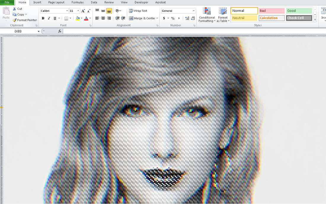
After a few tricks - such as finding the right order of the data stored - we’re able to convert the previous gibberish to pixel information/excel cell information. This is where putexcel gets good. The matrix of color information is passed to a Stata dataset so that it utilizes the fpattern cell expression of putexcel. An example Stata variable would look like this:

V1
A1=fpattern(“solid”, “234 243 243”)
A2=fpattern(“solid”, “234 243 243”)
A3=fpattern(“solid”, “234 243 243”)

Because we have a column of strings we can use the levelsof command to create a list containing each of these expressions and write them directly using the putexcel command. Now we’re ready to shake shake shake out that final command:

foreach v of varlist * {
        levelsof(`v'), local(`v') clean
        local cellexp = "`v' `cellexp'"
}

local cellexp = subinstr("`cellexp'", " ", "' ", .)
local cellexp = subinstr("`cellexp'", "v", "`v", .)
putexcel `cellexp' using "Art.xlsx", sheet("LoveStory") replace

The trick here is using the option "clean" in our levelsof command to strip all the double quotes so that we can use it directly in our putexcel statement. While we could have included the putexcel statement within the loop, the advantage here is that, because we’re only calling the command once, we don’t have to continually open and close the excel file for each putexcel statement - making it run in seconds. Now we’re ready to find our Starbucks lovers, get in fights at 2:30 am, and never ever get back together because we just saved ourselves so much time!

Can you spot all the Taylor Swift references? I count seven.

3 Comments

W=M/Stata

Welcome

HMAC-SHA1 in Stata

The Fuss

The SHA-1

The HMAC

The Conclusion

Just One More Binary Thing (I Promise)

On writing binary files in Stata/Mata

Stata's File Command

Mata's File Command

Mata's Buffered I/O Command

Reading the Files Back

Bits, Bits, Bits

Color Theory

Bitmap Structures

Writing Binary

Putexcel Part I: It’s No Picture to Burn

Author

Archives

Categories

W=M/StataWelcome

HMAC-SHA1 in Stata

The Fuss

The SHA-1

The HMAC

The Conclusion

Just One More Binary Thing (I Promise)

On writing binary files in Stata/Mata

Stata's File Command

Mata's File Command

Mata's Buffered I/O Command

Reading the Files Back

Bits, Bits, B﻿its

Color Theory​

​Bitmap Structures

Writing Binary

Putexcel Part I: It’s No Picture to Burn

Author

Archives

Categories

W=M/Stata

Welcome

Bits, Bits, Bits

Color Theory

Bitmap Structures