Why Care Block:
Yo yo, what’s up my Stata-ites! DJ Control+D is in the house because today we’re talking about making music with Stata. There’s a big trend in today’s age involving visualizations, but truth be told, visualizations are so last season. You’ve always been able to see your data, yet have you ever wanted to hear your data? “That’s absurd, I don’t need that.”
Yeah, you’re probably right... but today, this post is for the slacker: from the undergraduate struggling through their Stata homework, to the professional who’s bored with the day-to-day grind, our new command composer is there to brighten up your day and aid with your ever evolving procrastination techniques. What is composer? It’s a way to create music. How is that music generated? You write a string of notes that get converted to the midi file format. Why did we do this? I’m still asking myself that same question while introspectively reevaluating my life. Truth be told, I love music. Not in the traditional sense, but in the very traditional sense – classical music and music theory has always been a passion of mine and this has been a passion project for a long time now. 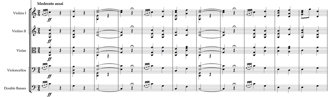
Composer makes music in two separate ways. You can write songs from the command line and from a dataset. The command line approach is faster and is especially meant for ad hoc procrastination. The dataset approach is a more methodical way of creating music and actually allows for multiple tracks and multiple instruments. Take our command line approach: composer "D, 384D, A, A, B, B, *2A, G, G, F#, F#, E, E, *.25r, *.25Db, 768D" using tt.mid, play replace We could have also written this first part as D, D, A, A, B, B, 768A, but it’s good to see the variations of this command. First we have notes: A, B, C, D, E, F, and G. Each note can be modified using a # (sharp) or a b (flat) which directly follows the note. A number before the note shows the duration of the note. The quarter note takes the value 384 (3*2^7). This way it can be halved up to seven times with 384 representing a quarter note, 192 representing an eight note, 96 a sixteenth note, and so on. Rather than specify a value, you may also multiply the note by a number to modify the value of the quarter note. Any number following your note denotes which octave or pitch your note will take. You may also change the instrument using a number or a named instrument available in the composer help file. For instance, say we wrote:
local n1 = "F#,A,E6,D6,E6,D6,A,D6"
local n2 = "E,A,E6,D6,E6,D6,A,D6"
local n3 = "F#,B,E6,D6,E6,D6,B,D6"
local n4 = "G,A,E6,D6,E6,D6,A,D6"
composer "`n1',`n1',`n2',`n2',`n3',`n3',`n4',`n4'" using ls.mid, play replace instrument("Pizzicato") bpm(240)
See if you can identify the song! Now take our data set approach. It’s just like the command line approach, except the command now takes sets of three variables: time duration, note, and octave. Notes can be played simultaneously by adding another track (three more variables). This way we can build chords and add volume to our masterpieces just like Beethoven. But unlike Beethoven, we’re not creating classical masterpieces, we’re recreating pop music. If you weren’t able to pinpoint the song before, here’s the dataset aided version of our previous track.
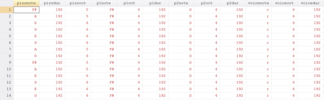
ls.dta Contents
use http://www.wmatsuoka.com/uploads/2/1/4/6/21469478/ls.dta, clear
composer pizzdur pizznote pizzoct p1dur p1note p1oct p2dur p2note p2oct voicedur voicenote voiceoct using ls.mid, play replace bpm(120) instrument(Pizzicato Pizzicato Pizzicato Voice)
And there we have it, a fairly easy way to write music in Stata. Is this interesting? I hope so, especially if you’ve made it this far. I’m sure you’re wondering how useful this is though. Truth be told, this is probably one of the only things on this blog that I haven’t found a general use for but perhaps you can find some sort of practical application and share your thoughts. There will be one more post about music soon which deals with the actual analysis of music which will use composer. Until then, good luck and stay creative future Stata maestros!
25 Comments
OAuthWhy Care Block:
Oh man, things are about to get real juicy – this is the final reveal of the Twitter API and I couldn’t think of a better time to do this. After all, we’ve made a complete mess out of Stata with our unruly bitwise operators, unending computer security algorithms, and un-um… unfortunate time-based C-plugins. Well, my Stata friends, this is how to do anything with Stata and the Twitter API.
Let’s post! Seriously, let’s tweet about things using Stata. This method can be used not only to tweet, but also to send direct messages, retweet things, and like (favorite) others’ tweets. If you’re like me, you don’t really use Twitter that well and I’m sure my 40 followers (I rounded up) would agree. But wouldn’t it be great to find a way to reach thousands of Twitter followers based off of hashtags or messages or even emoji? If the answer is no, fine, that’s my best attempt at convincing you but still feel free to read on. Let’s bring together everything we need to send a Tweet out on the internet:
Base64 Encoding
Easy way to turn readable stuff into unreadable stuff for humans but it’s not so bad for computers. This takes all alphanumeric characters plus the plus and the “/” (which equals 64 characters to choose from), converts 8-bit chunks into 6-bit chunks which end up receiving the specific character. Sometimes equal signs are added, but you already know that.
See post on Base64 Encoding Bitwise Operators and Security Methods
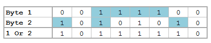
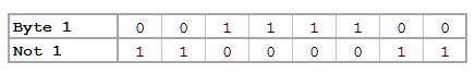
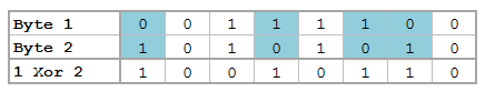
We’ve got bits dressed to the nines: shifting operators, rotating operators, logical operators, overflow methods, and all kinds of methods to translate from base 2 to base 16 to base 10.
These feed into our HMAC-SHA1 algorithm, which was awful to develop… this seriously has to go in the “lots of effort, little reward” category. See post on Bitwise Operators and HMAC-SHA1 Stata Plugins
We needed time - I mean we all do – in seconds since 1970 based off of Greenwich Time. We could have just accounted for our respective time zones (unless you’re located in GMT+0 of course), but why not use this as a great learning opportunity?
See post on Plugins Nonce
Once? None? Scone? What’s a nonce? Simply put, it’s a random 32 character word containing all alphanumeric symbols. Twitter’s example shows this being Base64 encoded, but all it has to be is a random string. vqib2ve89dOnTusESAS26Ceu9TcUES2i – see? Easy, just make sure you change the characters each time.
Percent Encoding
What%27s%20percent%20encoding%3F
Based on the UTF-8 URL Encoding standards, we need to replace certain characters that would otherwise cause complications in a URL. Don’t worry though, we’ve got a function for that. Just know that valid URL characters are all letters and numbers as well as the dash, the period, the underscore, and the tilde.
Send Out the Tweets
Twitter has some fabulous documentation for their API so it’s fairly easy to find the method that you want to do. These processes can be generalized and used across many of these methods so we are by no means limited to just tweeting. For tweets (hereon referred to as status updates to be consistent with Twitter’s documentation), we use the base or “resource” URL:
https://api.twitter.com/1.1/statuses/update.json Remember, status updates can only be 140 characters and Twitter will actually shorten URLs for you, but still keep in mind your character limits! All statuses must be percent encoded, so let’s go ahead and create our status local; we’ll also store our base URL while we’re at it.
local b_url "https://api.twitter.com/1.1/statuses/update.json"
local status = "Sent out this tweet using #Stata and the #Twitter #API – http://www.wmatsuoka.com/stata/stata-and-the-twitter-api-part-ii tells you how!"
mata: st_local("status", percentencode("`status'"))
We then take all of our application information: consumer key, consumer secret, access token, and access secret and store these as locals as well. local cons_key "ZAPp9dO37PnzCofN2Nm8n8kye" local cons_sec "kfbtARFpBIdb515iaS48kYZjWhLoIdbEiAINDVX0c3W3e0fgWe" local accs_key "1234567890-YFklDWGuvSIGLYPMnAfOZgLgLsMXjKIHqaIr1F5" local accs_sec "LYvHWfTS6LXjtDPVXchs6dXUG52l41j4HmicYwjr8aStw" For this section, we will be creating all of our necessary authentication variables. The first step to creating our secret signing key is to make a string that contains our consumer secret key, concatenated with an ampersand, concatenated with our access secret key. We’ll also include all the necessary locals we talked about earlier.
local s_key    = "`cons_sec'&`accs_sec'"
mata: st_local("nonce", gen_nonce_32())
local sig_meth = "HMAC-SHA1"
// If you don't make a plugin, just make sure you do seconds since 1970
// probably using c(current_date) and c(current_time) - [your time zone]
plugin call st_utm
local ts = (clock(substr("`utm_time'", 4, .), "MDhmsY") - clock("1970", "Y"))/1000
Now it’s time to create our signature. We start by percent encoding our base URL. For our signature string, we include the following categories:
local sig = "oauth_consumer_key=`cons_key'&oauth_nonce=`nonce'&oauth_signature_method=`sig_meth'&oauth_timestamp=`ts'&oauth_token=`accs_tok'&oauth_version=1.0&status=`status'" Then, percent encode the signature string and base URL:
mata: st_local("pe", percentencode("`b_url'"))
mata: st_local("pe_sig", percentencode("`sig'"))
This next step is why we spent an ungodly amount of time on bits and hashes! We need to transform our signature string into a Base64 encoding of the HMAC-SHA1 hash result with our message being the percent-encoded signature base hashed with our secret key. Sorry if that's a mouthful, but we can see what that translates to below.
local sig_base = "POST&`pe'&"
mata: x=sha1toascii(hmac_sha1("`s_key'", "`sig_base'`pe_sig'"))
mata: st_local("sig", percentencode(encode64(x)))
Finally, we’re almost done with Twitter and can move on to other more important things! First let’s make sure to post our Tweet because, after all, that's what we're here for. !curl -k --request "POST" "`b_url'" --data "status=`status'" --header "Authorization: OAuth oauth_consumer_key="`cons_key'", oauth_nonce="`nonce'", oauth_signature="`sig'", oauth_signature_method="`sig_meth'", oauth_timestamp="`ts'", oauth_token="`accs_tok'", oauth_version="1.0"" --verbose Now we can marvel at how much time we spent learning about something 99% of us don’t really care about. This is for you, 1% - this is all for you.
PS: Want to add emoji? Go to this site, find the URL Escape Code sections, and add the result to your status string! Ex: %F0%9F%93%88 = Chart with Upward Trend Bitwise Operators (aka Bits, Bits, Bits Part II)
Did you know that Mata supports bitwise operators? Well, it actually doesn't – in the typical sense. But that won't stop us from making it work. You see, Mata can handle data extremely well, and with a little finesse, can be forced to do things it wasn't really made to do. Yes it's going to be slow, and yes it's probably not very useful to the average user, but let me try to convince you how great using Mata really is!
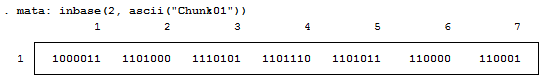
For those who don't know, Mata is a lower level language than Stata – many of Stata's complex functions are actually written in Mata because it's really quite fast. Mata mimics a lot of C's syntax, but also simplifies things so you don't feel like you have to explicitly declare everything. In previous posts we've exploited the power of the - inbase() - function and we will make ample use of that today. Say we have a text file containing the word "Chunk". While we see a word, the computer sees numbers which correspond to each letter – otherwise known as ASCII. Mata's - ascii() - function can help us find this representation: 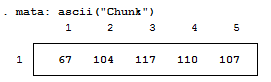
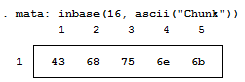
This is a simple way of converting our text into numbers, but how about into bytes? Typically, bytes are displayed in base 16:
But now we want to see each bit. Remember, I'm not a computer scientist, so you can trust me when I say this really isn't all that bad for those of you who haven't been exposed to this stuff. Just know that each of these bytes contains 8 bits. Each bit can either be on or off (1 or 0) which means that there’s a total possible bit combination of 2^8 = 256 per byte. Let's look at what Stata shows us when we look at everything in base 2:
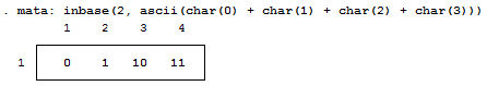
Notice, I added a zero and a one at the end of the text string "chunk" for illustrative purposes. Why are these values not 0 and 1 respectively? That’s because the digits are also ASCII characters (digits 48 and 49). We can get the values of zero and one by using the - char() - function. For fun, we'll also look at values two and three as well.
Well, because there are technically 8 bits per byte, we need to pad each output with zeros so that the total length is 8 bits. For example: the value "3" can be written as "11" in base 2, but is the same "00000011" so that we can imagine all 8 bits. We can easily accomplish this in matrix form.
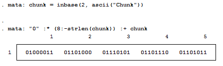
Notice the use of the colon operator? It's by far one of my favorite operands (not that I have that many) because it does the same operation on each element of the matrix, which makes the overall statement extremely succinct! The statement above just says: "Give me some zeros, exactly 8 minus how every many numbers we had, and append the original statement to the end to make sure every element has exactly 8 digits."
We should probably make this into a function, since we’ll use it a lot. So let's make the size of the padding an input as well.
mata:
string matrix padbit(string matrix x, real scalar padnum)
{
        string matrix y
        y = "0" :* (padnum :- strlen(x)) :+ x
        return (y)
}
end
mata: padbit(chunk, 8)
|
|||||||||||||||||
| bitwise-mata-functions.do |
Shifts and Rotations
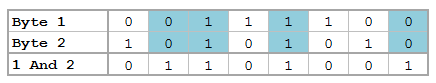
It's interesting to follow, though not all that interesting if it doesn't have a practical application. If you're like "honestly, I don’t know nothing about bit functions", I'll say - well I've got the one you. How about a way to easily encrypt your files so that you can hide your sensitive stuff in plain sight? First find a file and read it in:
// Read in File to Copy
fh  = fopen("Building an API Library.docx", "r")
eof = _fseek(fh, 0, 1)
fseek(fh, 0, -1)
x = fread(fh, eof)
fclose(fh)
Convert the file characters to the ASCII decimal value then convert this number into the base 2 representation (don't forget to pad the bits). From here, we can use our bitwise operations before converting this number back to base 10 and finally back to characters:
// Run Bitwise Not
y = padbit(inbase(2, ascii(x)), 8)
for (i=1; i<=cols(y); i++) {
        y[i] = bitnot(y[i])
}
y = char(frombase(2, y))
Lastly, write your newly altered file using Mata. This is obviously very basic, but a great way to hamper nosy coworkers.
// Write the Results to File
fh = fopen("Copy.docx", "w")
fwrite(fh, y)
fclose(fh)
But really, we're doing this with the ultimate goal of gaining access to Twitter data using Twitter's API. This is just step one of a three part series and if you're lost so far. there's plenty of time to see the motivation for this post in the next step. I promise it gets more interesting, yet I hope I've shown some of Mata's potential and how you can easily bring in the concepts to your own do-files.
On writing binary files in Stata/Mata
We start by making up a fake type of file called a wmm file. This file always begins with the hex representation ff00, which we know just means 255-0 in decimal or 11111111 00000000 in binary. The next 20 characters spell out “Will M Matsuoka File” followed by a single byte containing the byte order or 00000001 in binary. From there, the next four bytes contains the location of our data as we put a huge buffer of zeros before any meaningful data. It makes sense to skip all of these zeros if we know we don’t need to ever use them. After these zeros, we’ll store the value of pi and end the files with ffff.
The file looks like this:
Stata's File Command
tempname fh

file open `fh' using testfile.wmm, replace write binary

file write `fh' %1bu (255) %1bu (0)
file write `fh' %20s "Will M Matsuoka File"

file set `fh' byteorder 1
file write `fh' %1bu (1)

* offset 200
file write `fh' %4bu (200)

forvalues i = 1/200 {
        file write `fh' %1bs (0)
}

file write `fh' %8z (c(pi))
file write `fh' %2bu (255) %2bu (255)

file close `fh'
The only thing I feel I need to note here is the binary option under file open. Other than that, take note that we’re setting the byteorder to 1. This is a good solution to writing binary files; however, since most of my functions are in Mata, we might as well figure out how to do this in Mata as well.
Mata's File Command
mata:
fh = fopen("testfile-fwrite.wmm", "w")

fwrite(fh, char((255, 0)))
fwrite(fh, "Will M Matsuoka File")

// We know that the byte order must be 1
fwrite(fh, char(1))

fwrite(fh, char(0)+char(0)+char(0)+char(200))
fwrite(fh, char(0)*200)

fwrite(fh, char(64) + char(9) + char(33) + char(251) +
        char(84) + char(68) + char(45) + char(24))

fwrite(fh, char((0,255))*2)
fclose(fh)
end
I personally like the aesthetic of this syntax; it’s clean, neat, and relatively simple. The only problem is its ability to handle bytes. In short, it doesn’t do it at all. We’d have to build some more functions in order to accomplish this task (especially when it comes to storing double floating points) which is why Mata also has a full suite of buffered I/O commands. It’s a little more complicated, but well worth it. After all, we cheated in converting pi to a double floating storage point by using what we wrote in the previous command. This is not a good practice.
Mata's Buffered I/O Command
mata:
fh = fopen("testfile3-bufio.wmm", "w")

C = bufio()
bufbyteorder(C, 1)

fbufput(C, fh, "%1bu", (255, 0))
fbufput(C, fh, "%20s", "Will M Matsuoka File")

// We know that the byte order must be 1
fbufput(C, fh, "%1bu", bufbyteorder(C))

fbufput(C, fh, "%4bu", 200)
fbufput(C, fh, "%1bu", J(1, 200, 0))

fbufput(C, fh, "%8z", pi())

fbufput(C, fh, "%2bu", (255, 255))
fclose(fh)
end
The one distinction here is the use of the bufio() function. It creates a column vector containing the information of the byte order and Stata’s version, but allows us to use a range of binary formats available to use in Stata’s file write commands.
Reading the Files Back
mata:
void read_wmm(string scalar filename)
{
        fh = fopen(filename, "r")
        C = bufio()

        fbufget(C, fh, "%1bu", 2)
        if (fbufget(C, fh, "%20s")!="Will M Matsuoka File") {
                errprintf("Not a proper wmm file")
                fclose(fh)
                exit(610)
        }

        bufbyteorder(C, fbufget(C, fh, "%1bu"))

        offset = fbufget(C, fh, "%4bu")
        fseek(fh, offset, 0)

        fbufget(C, fh, "%8z")

        fclose(fh)
}

read_wmm("testfile-fwrite.wmm")
read_wmm("testfile.wmm")
read_wmm("testfile3-bufio.wmm")
end
And there you have it, a bunch of different ways to do the same thing. While I enjoy using Mata’s file handling commands for its simplicity, it does get a little cumbersome when writing integers longer than 1 byte at a time. Time to start making your own secret file formats and mining data from others.
First, let’s create a fake dataset with help from Nick Cox’s egenmore ssc command:
set obs 300
forvalues i = 1/200 {
        gen x`i' = round(runiform()*50*_n)
}

gen id = _n
reshape long x, i(id) j(vars)
egen count = xtile(x), nq(30)
keep id vars count
Today we will be making a bitmap of a map for Fitbit activities by writing bits of binned colors in a binary file. Alliteration aside, this post pulls from various sources and is intended to cover a great deal of topics that might be foreign to the average Stata user – in other words, hold on tight! It’s going to be a bumpy bitmap ride as we cover three major topics: (1) Color Theory, (2) Bitmap Structures, and (3) Writing Binary Files using Stata.
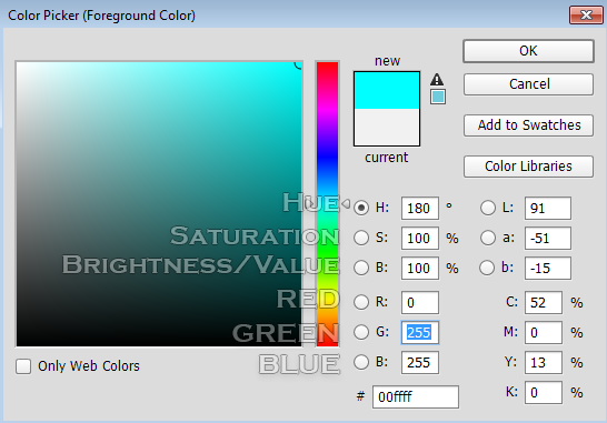
Color Theory
Bitmap Structures
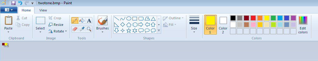
For simplicity’s sake, the only things we'll need to change are the numbers of rows and columns in the bitmap header.
As for the body, there are three rules we need to keep in mind here:
- The picture starts in the lower left-hand corner, reading right to left. If you forget to do this, your picture will be vertically flipped.
- The bytes are written in the opposite order for colors: instead of writing in RGB, you need to write in BGR.
- All “columns” need to be divisible by four. You need to add zeros as a buffer until your column is divisible by four.
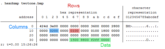
. mata: inbase(16, 500)
  1f4
Let’s add a zero in front of that to get 01f4 as our width. Once again, we must reverse this order; therefore, our real values to write are f4 and 01. Converting these values using frombase() yields 244 and 1 respectively. These are the bytes we’ll end up writing in the next section.
Writing Binary
My code broke out this task in two sections: writing the header and writing the body:
The Header
The header is fairly straight forward: just copy and paste the hexdump from before (converting from base 16 to base 10) or by reading in the file byte by byte.
file open myfile using testgrad.bmp, write replace binary
file write myfile %1b (66) %1b (77) %1b (70) %1b (0) %1b (0) %1b (0)
file write myfile %1b (0) %1b (0) %1b (0) %1b (0) %1b (54)
file write myfile %1b (0) %1b (0) %1b (0) %1b (40)
file write myfile %1b (0) %1b (0) %1b (0)

mata: bitmap_rowcol(bitmap_size(200), bitmap_size(300))
file write myfile %1bu (`c1') %1bu (`c2') %1bu (0) %1bu (0)
file write myfile %1bu (`r1') %1bu (`r2') %1bu (0) %1bu (0)

file write myfile %1b (1) %1b (0) %1b (24)
file write myfile %1b (0) %1b (0) %1b (0) %1b (0) %1b (0) %1b (16)
forvalues i = 1/19 {
        file write myfile %1b (0)
}
Notice the order of the column and row variables. I create these values using the separate function bitmap_rowcol() to deal with the problem mentioned earlier. Think of `c1’ as 244 and `c2’ as 1, and `r1’ as 2c and `r2’ as 1 for a width of 500 pixels and a height of 300 pixels with rules according to our previous analysis.
The Body
From there, we call bitmap_body in mata and close our file (cols is 200 in my example)::
mata: bitmap_body(${cols}, X, buff)
file close myfile
This is all great, but I’m not going to lie, it means absolutely nothing to me without seeing the final result. So here it is:

HSV Gradient with a 5 px Gaussian Blur
|

RGB Gradient with a 5 px Gaussian Blur
|
| bitmap.do |
Author
Will Matsuoka is the creator of W=M/Stata - he likes creativity and simplicity, taking pictures of food, competition, and anything that can be analyzed.
For more information about this site, check out the teaser above!
Archives
July 2016
June 2016
March 2016
February 2016
January 2016
December 2015
November 2015
October 2015
September 2015
Categories
All
3ds Max
Adobe
API
Base16
Base2
Base64
Binary
Bitmap
Color
Crawldir
Email
Encryption
Excel
Exif
File
Fileread
Filewrite
Fitbit
Formulas
Gcmap
GIMP
GIS
Google
History
JavaScript
Location
Maps
Mata
Music
NFL
Numtobase26
Parsing
Pictures
Plugins
Privacy
Putexcel
Summary
Taylor Swift
Twitter
Vbscript
Work
Xlsx
XML
 RSS Feed