Why Care Block:
Let’s be clear, I really like Stata graphics! There are people out there that complain about Stata graphics not looking flashy enough, but this is a really good thing – you have to know enough about the Stata graphics suite to make a graph look as bad as many new-excel-user graphs. “Let’s add drop shadow, 3D, hovering label boxes, gradients, and lots of pictures” is a good idea when you’re the van Gogh of graphics, but most of these graphs end up resembling more of a Picasso leaving the audience asking whether that’s a y-label, or a text box, or maybe even an eye…
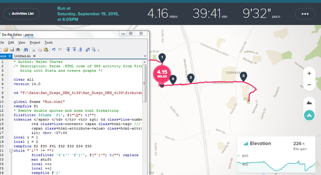
You may have noticed that there’s been a significant gap in these posts over the last few months and it’s been completely intentional. My talented friend, Belen, and I have been studying Stata graphics enough to be labeled as completely crazy, but at least it has resulted in a marvelous presentation for the Stata User Group meeting. This process involves a lot of JavaScript and Stata integration to produce Tableau-like interactive graphs using the same familiar syntax that all Stata users know and love. However, that’s not what we’re talking about in this post, no, get ready because today we are switching to graphic design with help from Adobe’s Creative Cloud! Look, all math and no art makes for some REALLY boring posts – and we strive to make sure no post is too boring. So we’ll spice things up by combining fitness, art, and math into one! Before we go any further, if you’d like to follow along you might need to get yourself a copy of Adobe Illustrator CC which comes with a free 30-day trial. Adobe Illustrator is a lot like the more commonly known Photoshop, but it specializes in making some really cool vector graphics. You know, logos, drafts, general art. Did you know that all Adobe products can be scripted using AppleScript, VBScript, and JavaScript? Today, we’ll take advantage of very simple JavaScript statements in order to beautify our data. Our example data for this post comes from the aforementioned Fitbit API. Belen and I both ran two half-marathons this year: the San Diego Half, the La Jolla Half, and the Rock ‘n’ Roll Half. Yes, there’s three halves here, that’s because we ran two separately and one together! While I’m very proud of our accomplishments, there’s a goldmine of data from our Fitbits just waiting to be visualized. Each Fitbit activity contains time, distance, location, heart-rate data and more. First things first, because the races started at different dates and different times, we should standardize our time variable (clock) to be time since the first gun start. gen time = clock - clock[_n-1] replace time = sum(time) duplicates drop time, force
We do this for both datasets, we’ll call them WM and BC. We’ll also preface all variables with the prefix WM or BC before we merge the data. This can easily be accomplished by the command:
ren * WM*
ren WMtime time
Now we can merge the WM set on the BC set and standardize.
collapse (max) WM* BC* time, by(Time)
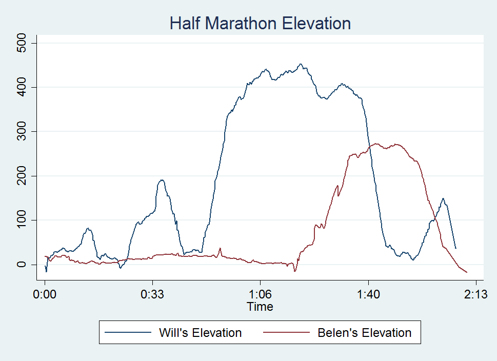
line WMelevation BCelevation Time
Look at that, a perfect 2D representation of our halves on the same axis. The x-axis measures distance and time to completion whereas the y-axis shows the elevation at that time. A steeper slope shows a very quick climb. This is my one issue with this type of graph, it doesn’t show just how grueling the La Jolla Half once you enter Torrey Pines National Park, but what doesn’t kill you makes you stronger.
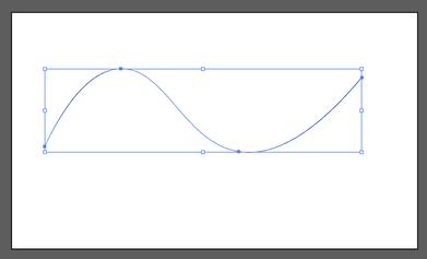
Now, if you know about Adobe products but haven’t used any scripting yet, you’re in for a treat! With Adobe CC you can easily download the Adobe ExtendScript Toolkit IDE from the Creative Cloud, and this will allow us to do all of our scripting. Unfortunately, many of you might know of easier ways to do what we’re going to accomplish in the next step so I have to mention this is merely for informative purposes that serves to remove the roadblock of knowing how to integrate Stata with Adobe products. Back to the tutorial, let’s take this path for instance:
It has four anchor points at some set of coordinates in our drawing space. The coordinates usually take the form (x,y) so we can think of our path as an array of four coordinates. Let’s look how we might start creating this path in JavaScript:
var doc = app.activeDocument;
var stataPath = new Array(4);
Here, we set up our document as a variable as well as the path we’re going to create. Notice, the path is going to be an array with four elements. We start coding the elements as such (remember JavaScript lists initialize at 0): stataPath[0] = new Array(78 , 317); stataPath [1] = new Array(258 , 133); stataPath [2] = new Array(537, 330); stataPath [3] = new Array(828 , 154); Finally, we just have to add the following lines to have it actually draw our shape! app.defaultStroked = true; newPath = app.activeDocument.pathItems.add(); newPath.setEntirePath(stataPath); And that’s essentially it! I usually have Stata write the data I need to these arrays and enjoy how easy it is to create artful representations of our otherwise technical graphs. One quick note, you should probably transform your data so that it fits in the dimensions of your Illustrator file (or you can scale it later). Writing our script is extremely simple with the use of –filefilter – and loops.
tempfile f1
file open myfile using `f1', write replace
forvalues i = 1/`=_N' {
        file write myfile " stataPath [`=`i'-1'] = new Array( `=Time[`i']' , `=`init'[`i']');" _n
}
file close myfile
view `f1'
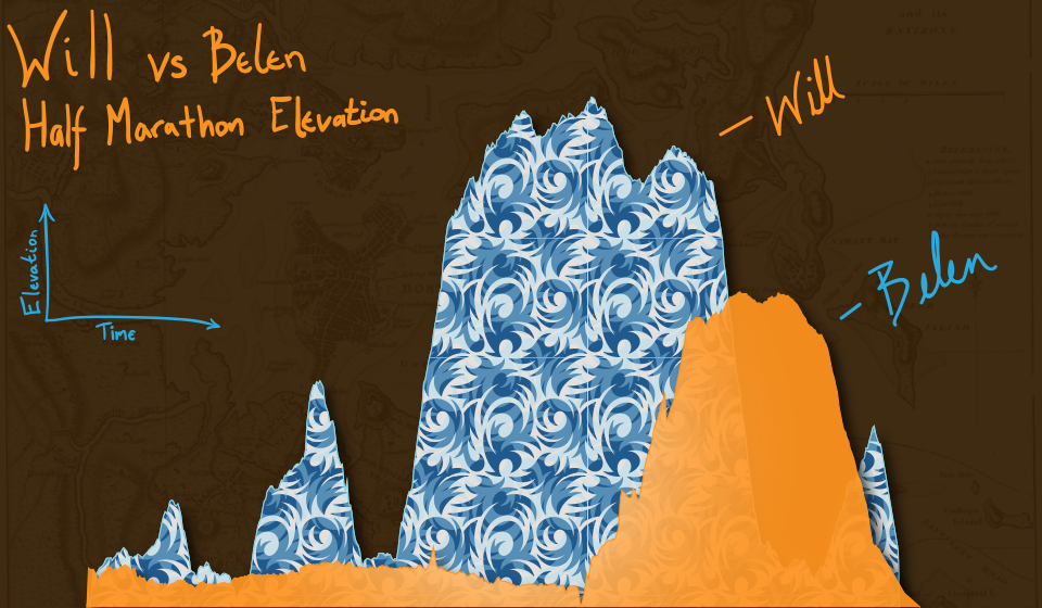
Once you run your script, the math stuff is over and it is time to make art! Happy drawing. In an unrelated note, the second reason for the lack of posts is because Belen has recently moved from San Diego and I wanted to take a moment to thank and acknowledge her for her contributions to wmatsuoka.com. She’s been my unofficial editor and a great soundboard for what ideas are too stupid to make the cut for the Stata blog. While it is always sad to see someone go, I wish her all the best in her new endeavors. Good luck, Belen! And here’s the final result of our blog: be forewarned that I am not claiming to be an artist.
5 Comments
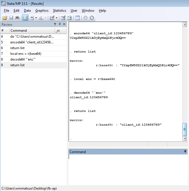
Why Care Block: Happy New Year! We're starting 2016 with a bang, including this three part series on acquiring Fitbit data through Fitbit’s API services. 2015 was a great year and marked the start of this website, and I can guarantee that there will be much more content to come. See the new "Why Care Block"? It’s inspired by a Holiday conversation with family and gives a brief synopsis of why we’re even doing this in the first place. With that, let's talk about the topic of the day: Base64 encoding. Base64 encoding exists for some privacy purpose. That's about all I want to say about Base64 encoding. Let's just look at an example, they’re a lot cooler. Say for instance we have the phrase: “This is kinda boring…” By converting every character to ASCII bytes (and by potentially adding padding), converting each byte to base 2, taking the 8-bit representation of the binary character and convert it to a six bits, converting that back to base 10, and using those numbers (they fall between 0 and 63) to look up the corresponding character of the alphabet plus two other characters, we finally arrive at the following encoded string: "VGhpcyBpcyBraW5kYSBib3JpbmcuLi4=" While they mean the same thing, I think the first phrase was a little more accurate. We can encode this second phrase a second time and it gives us: "VkdocGN5QnBjeUJyYVc1a1lTQmliM0pwYm1jdUxpND0=" Now you can easily send encoded messages to your friend (not plural – I can't imagine that many people would tolerate this type of behavior). I’ve put together a Stata package containing these routines; however, no help file is available upon the first release. Here is a brief overview of the new commands, encode64 and decode64 at work. We first called encode64 on the string "client_id:123456789" to encode this value in Base64. The result shows under the command, but is also callable through the macro r(base64). We create a local macro that contains this encoded value ("Y2xpZW50X2lkOjEyMzQ1Njc4OQ==") and decode this message to get back to our original string. It's a lot less fun than my old Nintendo 64, but trust me, the results will be extremely rewarding! Feel free to download the ado file below.
Coercion. It’s the topic of the day, and a short topic at that. Coercion is the leading driver for Excel usage for most Stata users. Workbook linkage is usually a pain – the practice of linking one cell from a workbook to a different cell in another workbook – and can turn a relatively simple task into a nightmare usually ending the job with a headache and a stiff drink.
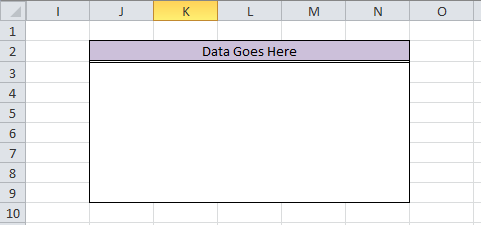
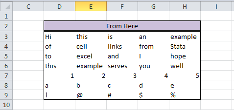
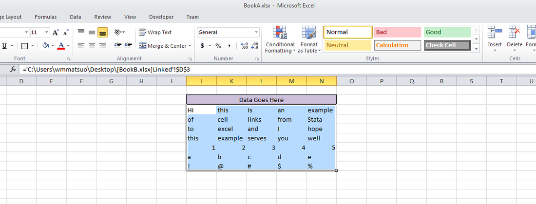
However, with a few simple Mata commands, the crisscross of equal signs, dollar signs, and formulas can turn a repetitive task into a few simple copy-and-paste commands. There is also less room for error. For fun, we'll do this entire thing in Mata. First, we need to decide how many observations/variables we need. Let’s look at our current workbook and target workbook.
So we need 5 columns and 7 rows, with columns from D to H and rows from 3 to 9 in our BookB set. Write it:
mata:
st_addobs(7)
st_addvar("str255", "v" :+ strofreal(1..5))
Starting with a blank dataset, add seven observations. From there, we create 5 variables (v1 v2 v3 v4 v5) that are all of type str255. This is a placeholder value for long equations. The second part of this command “v” :+ strofreal(1..5) is my favorite part about Mata. The colon operator (:+) is an element-wise operator that is super helpful. No more Matrix conformability errors (well maybe a few). It creates the matrix:
("v1", "v2", "v3", "v4", "v5")
without much work and allows for any number of variables! Sidenote – changing (1..5) to (1..500000) took about 3 seconds to create 500,000 v#’s. Next, let’s set up our workbook name: bookname = "'C:\Users\wmmatsuo\Desktop\[BookB.xlsx]Linked'!" Specify the location of the workbook with the file name in square brackets and enclose the sheet name in apostrophes. End that expression with an exclamation point! Since we know we want D through H, and cells 3-9, we can write the following: cols = numtobase26(4..8) rows = strofreal(3::9) numtobase26() turns 4 through 8 into D through H. For more information see my previous post on its inverse. The rows variable is a column vector containing values 3 through 9. Now it’s time to build our expression: expr = "=" :+ bookname :+ "$" :+ J(7, 1, cols) :+ "$" :+ rows We put an equals sign in front of everything so that Excel will know we’re calling an equation. Follow that with the workbook name. If you didn’t know, dollar signs in excel will lock your formulas so they don’t move when you copy formulas from one cell to another. We’ll put those in as well. The next part, J(7, 1, cols), takes our column letters and essentially repeats it seven rows down. Thanks to the colon operator, we just have to add another dollar sign to all elements of the matrix and our row numbers. Since the new cols matrix contains seven rows, and our row vector contains seven rows, it knows to repeat the row values for all columns. Let’s just put that matrix back into Stata and compress our variables.
st_sstore(., ("v" :+ strofreal(1..5)), expr)
stata("compress")
end
And voilà, we have a set of equations ready to copy into Excel. One quick tip: set your copy preferences so that when you copy the formulas, you won’t also copy variable names by going to edit->preferences->data editor-> uncheck “Include variable names on copy to clipboard”. Now just copy the equations directly from your Stata browse window into Excel, and enjoy those sweet results! In other news, this post built upon the putexcel linking discoveries found over at belenchavez.com - who recently had her Fitbit stolen! Follow her journey to get it back on her website or on Twitter - hopefully she'll be able to coerce the thief into returning the device.
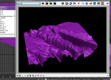
Some of the best ideas are those that happen right outside of your comfort zone. Unfortunately, they can also lie outside of your current means as well. Not to worry though, because with a little luck and a lot of perseverance, we can eventually erode away at the mountainous tasks that lie ahead. Like a running stream we can… well, perhaps that’s quite enough nature metaphors, but I think you get the picture. I’m personally extremely excited to reveal this next set of blog posts because it ties together so many different concepts. This means that it will be broken out into several different parts. However, the complexity also comes at a cost. I thought I would be done by now – the struggle is real! While I continue to do my research, I’ve added a quick snippet of what’s to be expected: Alright, so it’s not that exciting. Yet. Remember what I said about current means? 3D rendering takes quite a long time, and my current computer can’t handle it that well which means I’ll be upgrading (or borrowing) resources. I’d like to point out the silver lining within this video though – this is actual data for elevation and location. Stata wrote this. Stata also wrote these mountains below. With some help from an excellent source, Stata is able to bring in Fitbit data with ease. Finally, here’s a panorama picture from inside my pocket. It plays a big role in the posts to come... Stay tuned!
|
AuthorWill Matsuoka is the creator of W=M/Stata - he likes creativity and simplicity, taking pictures of food, competition, and anything that can be analyzed. Archives
July 2016
Categories
All
|
||||||


 RSS Feed