|
I was extremely lucky to receive an advanced copy of gcmap written by the folks over at www.belenchavez.com. You see, gcmap is an excellent program that uses Google Charts API to create professional web quality charts using your Stata datasets. Don’t believe me? Check out this example below.
Every NFL team, every NFL stadium, with pictures! This dataset was created by using information from Wikipedia. I’ve taken my fair share of stuff from Wikipedia, but I’ve also donated every year to the Wikimedia foundation, and you should too!
Today is December 13, 2015 – which also marks Taylor Swift’s 26th birthday. Happy Birthday, Taylor! In an extension to NFL stadiums, I’ve merged data from all the North American locations Taylor Swift played at in her 1989 World Tour. Here’s another example of how you can use gcmap in order to produce some great (although somewhat creepy) maps.
Enjoy - I hope we see a lot more Stata + Google Charts in the months to come!
Next up: NFL Injuries – an Artistic Approach
2 Comments
"Perhaps you've noticed the new Microsoft Office formats" is something you'd say back in 2007. Nevertheless, I'd bet that a good portion of people haven't looked into what that new "x" is at the end of all default files (.docx, .xlsx, .pptx) and an equal number of people probably don't care. However, I'd like to try and convince these doubters just how great this is! This "x" stands for XML (extensible markup language) and makes the file formats seem hipper than their x-less counterparts. Rather than documents and spreadsheets being stored as binary files, which are difficult to read, all information is stored in easily read zipped-xml files. That's right - all .abcx files are just zip files.
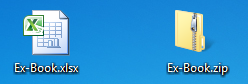
Let's look at an example Excel file (Ex-Book.xlsx):
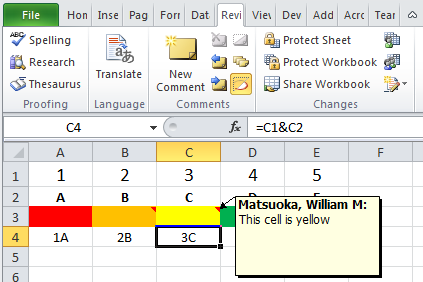
It has a little bit of everything: values, text, color formats, comments, and formulas. If we wish to look at how the data are stored, we can easily change the extension of the file from .xlsx to .zip.
Naturally, we already have a way to take care of zip files in Stata with the command unzipfile. So from this point on, we're going to navigate this file strictly using Stata. My Excel workbook is located on my desktop, so let's unzip it.
cap mkdir unzipbook cd unzipbook unzipfile ../Ex-Book.xlsx, replace dir xl/ 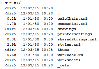
Note that we didn't have to change the extension, and we now have a list of files and directories under the "xl" folder. Files and properties of interest:
These are good reference files, but our main interest is located within the "worksheets" directory under our "xl" folder. Here, we can find each sheet named sheet1, sheet2, sheet3, etc. The sheets are indexed according to the workbook.xml files (ex: "rId1" corresponds to sheet1). I've always had trouble getting formulas out of Excel. Instead of resorting to VBA, we can now use Stata to catalog this information (I've found this very useful for auditing purpose). Here's a snippet of our worksheets/sheet1.xml file: 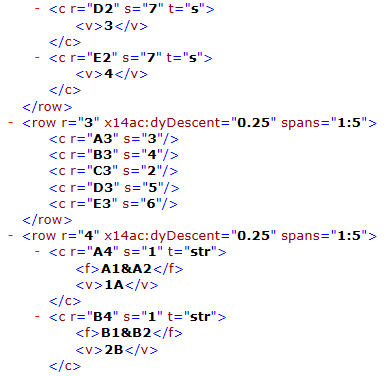
Interpreting this section, we can see that it contains rows 2-4 which corresponds to our strings (A, B, C), our styles (Red, Orange, Yellow), and our formulas. Going from top to bottom, by deduction we can see that our first <c> or cell class contains a value of 3 and references cell D2 with the style of 7. Here, since the type is a string ("s"), we need to reference our sharedStrings.xml file to see what the fourth string is. We look for the fourth string, since the count initializes at zero rather than looking at the third string. Our fourth observation is a "D" and our fifth observation is an "E" in the shareStrings.xml file.
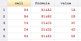
The third row contains our colored cells without any data. Therefore, they have no values, but contain styles corresponding to the fill colors. A quick note: the order here goes (3, 4, 2, 5, 6) because I accidentally chose yellow first. Finally, the most valuable part of this exercise (for me at least) are the formulas. Cell A4 contains the formula "=A1&A2" and displays the evaluated value of the formula. When linking to other workbooks, the workbook path will likely be another reference such as [1], [2], [3], etc. A quick use of some nice Stata commands below yields a simple code for creating an index of your workbook's information.
tempfile f1 f2
filefilter xl/worksheets/sheet1.xml `f1', from("<c") to("\r\n<c")
filefilter `f1' `f2', from("</c>") to("</c>\r\n")
import delimited `f2', delimit("@@@", asstring) clear
keep if regexm(v1, "([^<>]+)")
gen value = regexs(1) if regexm(v1, "v>([^<>]+)")
replace formula = subinstr(formula, "&", "&", .)
keep cell formula value
Thanks to that little x, we are able to easily obtain meta-information about our Excel files, presentations, or even Word documents. Think about having to look through thousands of documents to find a specific comment or reference - seems like a simple loop would suffice. Maybe that x is pretty cool after all.
With the release of Stata 14.1, Stata made a good amount of changes to one of my favorite commands: putexcel – I have mixed feelings about this.
First, I want to take the opportunity to stress version control. Always begin your do-files with the version command. If you don’t, you’ll likely get the error r(101) “using not allowed” when trying to implement your old putexcel commands in a do-file. A quick note about version: you must run this command with the putexcel statement. Just having it at the top of your do-file and calling it doesn’t work, unless you run the do-file all the way through. Think of using version control like using a local macro. What I like:
Putexcel has been simplified…
…but it requires changing the way you think about putexcel. Think of the command in a more modular structure.
Example:
putexcel set MyBook.xlsx, sheet("MyData")
putexcel A1=("Title of Data") A2=("Subtitle") A3=formula("SUM(A4:A20)"), bold
putexcel A3:A20, nformat(number_sep) hcenter
.
The updated options simplify your code a bit: No more bold(on), rather just bold or nobold and there’s no need for that modify command. Update: as of the December 21st update, modify is an option again... Advanced number formats may be used: No more restrictions, the advanced number format can now be used and can be found under putexcel advanced – which makes sense since it was able to be used already in the Mata xl() object. 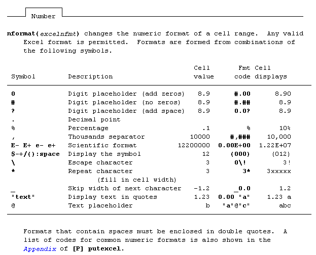
putexcel set MyBook.xlsx, sheet("MyData")
putexcel A3, nformat(#.000) nobold border(all)
What I don't like:
Using not allowed! I liked the using statement within putexcel, especially when I needed to add something as simple as a title on an excel spreadsheet. Now, I have to use two lines of code instead of one. This is a minor complaint compared to the next section.
The new syntax – it’s very difficult to work with large files, which is why I’ll be sticking with my “version 14.0” command when writing putexcel statements to large excel files. Why? I cannot find a simple way to write different format-types in one statement (say bold font in cell A1 and a border around cell B2). I have to do this in two separate commands. This is a big problem when you’re working with large excel files because Stata keeps opening the file, saving it, and closing the file for EVERY putexcel statement. We could waste minutes writing borders and adding different colors. Granted, Excel files shouldn’t be 40MB but we have them; and management wants to keep them that way, putting the Stata programmer between a rock and a hard place. Check out my previous post on “block” putexcel for working with very large excel files. What I hope happens:
We get the best of both worlds – the putexcel set keeps the Excel file open, so that it doesn’t continuously save file after file but the new format stays. If we have a putexcel set, why not putexcel close? Oh, and using is added back as an optional/hidden feature of putexcel. That, my friends, would be my ideal putexcel command: not too hot, not too cold; simple, yet powerful.
On writing binary files in Stata/Mata
As a supplement to my most recent posts, I decided to put together a quick guide on writing and reading binary files. Stata has a great manual for this – however, I struggled to see how this works in Mata. I spent a good afternoon scouring Google, Stata Journals, and Statalist to no avail. Little did I know, I was looking in the wrong places and for the wrong commands. It wasn’t until I broke out my old Mata 12 Mata Reference guide that I realized the solutions lie not with fopen(), but with bufio() (and yes, bufio() is referenced in fopen() - always check your references)
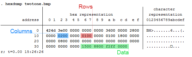
We start by making up a fake type of file called a wmm file. This file always begins with the hex representation ff00, which we know just means 255-0 in decimal or 11111111 00000000 in binary. The next 20 characters spell out “Will M Matsuoka File” followed by a single byte containing the byte order or 00000001 in binary. From there, the next four bytes contains the location of our data as we put a huge buffer of zeros before any meaningful data. It makes sense to skip all of these zeros if we know we don’t need to ever use them. After these zeros, we’ll store the value of pi and end the files with ffff. The file looks like this: Stata's File Command
tempname fh

file open `fh' using testfile.wmm, replace write binary

file write `fh' %1bu (255) %1bu (0)
file write `fh' %20s "Will M Matsuoka File"

file set `fh' byteorder 1
file write `fh' %1bu (1)

* offset 200
file write `fh' %4bu (200)

forvalues i = 1/200 {
        file write `fh' %1bs (0)
}

file write `fh' %8z (c(pi))
file write `fh' %2bu (255) %2bu (255)

file close `fh'
The only thing I feel I need to note here is the binary option under file open. Other than that, take note that we’re setting the byteorder to 1. This is a good solution to writing binary files; however, since most of my functions are in Mata, we might as well figure out how to do this in Mata as well. Mata's File Command
If you didn’t know, Mata’s fopen() command is very similar to Stata’s file commands, with a few slight differences that we won't touch on here. Just know, it's pretty awesome and don't forget the mata: command!
mata:
fh = fopen("testfile-fwrite.wmm", "w")

fwrite(fh, char((255, 0)))
fwrite(fh, "Will M Matsuoka File")

// We know that the byte order must be 1
fwrite(fh, char(1))

fwrite(fh, char(0)+char(0)+char(0)+char(200))
fwrite(fh, char(0)*200)

fwrite(fh, char(64) + char(9) + char(33) + char(251) +
        char(84) + char(68) + char(45) + char(24))

fwrite(fh, char((0,255))*2)
fclose(fh)
end
I personally like the aesthetic of this syntax; it’s clean, neat, and relatively simple. The only problem is its ability to handle bytes. In short, it doesn’t do it at all. We’d have to build some more functions in order to accomplish this task (especially when it comes to storing double floating points) which is why Mata also has a full suite of buffered I/O commands. It’s a little more complicated, but well worth it. After all, we cheated in converting pi to a double floating storage point by using what we wrote in the previous command. This is not a good practice. Mata's Buffered I/O Command
Let's get right to it
mata:
fh = fopen("testfile3-bufio.wmm", "w")

C = bufio()
bufbyteorder(C, 1)

fbufput(C, fh, "%1bu", (255, 0))
fbufput(C, fh, "%20s", "Will M Matsuoka File")

// We know that the byte order must be 1
fbufput(C, fh, "%1bu", bufbyteorder(C))

fbufput(C, fh, "%4bu", 200)
fbufput(C, fh, "%1bu", J(1, 200, 0))

fbufput(C, fh, "%8z", pi())

fbufput(C, fh, "%2bu", (255, 255))
fclose(fh)
end
The one distinction here is the use of the bufio() function. It creates a column vector containing the information of the byte order and Stata’s version, but allows us to use a range of binary formats available to use in Stata’s file write commands. Reading the Files Back
Now that we’ve written three files, which (in theory) should be identical, let’s create a Mata function that reads the contents stored in these files. Note: it should return the value of pi in all three cases. As it turns out, they all do.
mata:
void read_wmm(string scalar filename)
{
        fh = fopen(filename, "r")
        C = bufio()

        fbufget(C, fh, "%1bu", 2)
        if (fbufget(C, fh, "%20s")!="Will M Matsuoka File") {
                errprintf("Not a proper wmm file")
                fclose(fh)
                exit(610)
        }

        bufbyteorder(C, fbufget(C, fh, "%1bu"))

        offset = fbufget(C, fh, "%4bu")
        fseek(fh, offset, 0)

        fbufget(C, fh, "%8z")

        fclose(fh)
}

read_wmm("testfile-fwrite.wmm")
read_wmm("testfile.wmm")
read_wmm("testfile3-bufio.wmm")
end
And there you have it, a bunch of different ways to do the same thing. While I enjoy using Mata’s file handling commands for its simplicity, it does get a little cumbersome when writing integers longer than 1 byte at a time. Time to start making your own secret file formats and mining data from others.
You’re being tracked – in the world we live in today, almost everything you do has some sort of digital trace. I recently went to True North Tavern in North Park (San Diego) to mourn yet another 49er defeat – and to my surprise, they had a bouncer at the door checking IDs. I’ll admit, I am very lax in giving out my ID to anyone who asks for it, but on this occasion I did hesitate to provide identification a little as I saw a big black machine right by the door. Luckily, I made it through after a quick glance but as it turns out, a few friends were not so lucky. Besides visually checking ID’s the bouncers sometimes scan driver’s licenses into these black machines, which stores the patron’s driver’s license information including the photo! Today, we will explore why this is a very bad practice as we transition to talking about Exif data.
Exif, or exchangeable image file format, is a way to store information on your images or audio file. If you have an iPhone, you will probably notice that you can actually view your images on a map, and it shows you where and when you took the picture. This is really neat, especially if you’re a photo editor and need to match light or camera settings in Photoshop without having access to the physical camera. However, this is also incredibly dangerous. Here is a quick look at the properties of a photo I took with my iPhone 5. 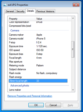
You can see everything, including the exact location of where I took the picture. Now, I’m sure this is not all that shocking, but it can be a little nerve wracking when you post pictures online knowing that someone can easily trace back where you were with a click of a button. Luckily, many social media websites such as Facebook and Twitter are aware of this and will strip your picture’s Exif data for you.
Exif data are stored in the header of your picture. What the heck does that mean? Every picture contains a header, and most new cameras and cell phones will actually write this data in the header. Your computer then reads this information and is able to tell your location, camera settings, and time stamps of the photo. One section actually contains all of the Exif tags – it’s really just a collection of information. In order to read this information, we have to read in the picture file which is a series of zeros and ones. Yup, we’re using Mata’s bufio() functions to read in all of this information. Bufio() allows us to write not only string characters, but also binary integers into files without using Stata’s file command. I will bore you with the details in a subsequent post, but for now, I’d like to introduce my program – exiflatlon – which strips JPG, TIF, and WAV file formats of latitude and longitude information. It can be used in two ways:
Let’s try out the directory specification.
exiflatlon, dir("C:\users\wmmatsuo\desktop")
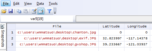
In the event there is no exif information, exiflaton will provide you with a warning and will replace those latitude values and longitude values with zeros in the resulting dataset. It only takes milliseconds to rip the locations off each photo – and this is valuable information, especially if you don’t want the wrong type of people (or really anyone) tracking you. While I only use Stata for good, there are likely people who use it for bad purposes. Only joking, Stata users are never malicious, but there are plenty of other programmers who are and who have more efficient tools at their disposal for such (and maybe creepier) purposes. In today’s age, we need to be careful about safeguarding our data because there are no moral boundaries when it comes to taking data. Companies love information, and will not hesitate to steal this information. After all, hiding the fact that “by entering this premise, you consent to us taking all your information from your ID” is in no way consent when it’s not clearly stated. I’m looking at you, True North Tavern...
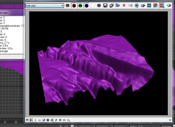
Have you ever been burdened with making up data? Of course not, you say! How dare you charge me with such accusations! Well first, calm down. Sometimes it’s okay to “make up” data. For instance, for testing purposes: perhaps you have an idea of the approximate shape of the data you’ll be feeding into your program, but some lazy programmer isn’t providing you with the necessary steps to proceed. You could create a sinusoidal function to create an approximate representation, but who really has the time for that. The solution lies with a 3rd grader’s doodle.
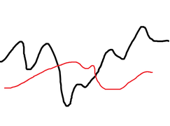
Balderdash! But really, it’s much easier to draw out the shape of your data that to input it cell by cell or create some function that’s going to be scrapped in the end anyway. Even better, perhaps someone put this graph in a presentation, but is refusing to share their base data. No problem for us. For this tutorial, we’re going to need to download GIMP, a free graphics editing software program that’s similar to Photoshop, but also drives me crazy because it has completely different hotkeys.
Take this image and open it in GIMP. Then make sure to save it as an HTML webpage. By selecting this option, GIMP converts every pixel to a cell in an HTML table, allowing for us to parse this information out ourselves. Remove HTML tags and only keep relevant information: each <td> tag should have a background color which is the hexadecimal RGB color of the cell. Recall that <td> tags indicate cell data whereas <tr> tags indicate a new row. Since each line contains a new bit of information, we don’t really care about the td tags. In fact, tag the <tr> tags (gen trtag = regexm(lower(v1), “<tr”), and take the running sum of that variable (replace trtag = sum(trtag)). This way, we have a corresponding row to each point of data. Create a running count variable by each row - this will give us column positions. Create a variable that’s equal to our column position gen black = run_count if y == "000000" gen red = run_count if y == "ed1c24"
Finally, collapse your black and red variables by your column variable: collapse black red, by(colpos) fast To make everything look nicer, I used the lowess command to smooth out my lines, but you don't have to if you're looking to get extremely accurate data. lowess black s, bwidth(.08) gen(bsmooth) lowess red s, bwidth(.08) gen(rsmooth)
* s represents our row count variable (trtag)
Finally resulting in: line *smooth s, lwidth(thick thick)
which gives us the following output in Stata:
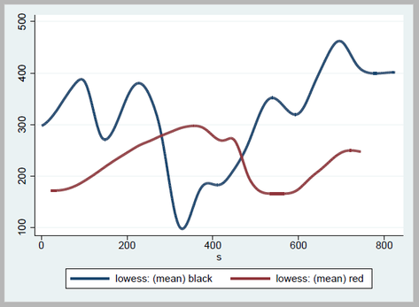
PLEASE NOTE: Stealing graphs and making up data are bad practices. I wouldn't actually do this in the professional setting. This post merely serves to show how this process may be done. I recently celebrated my Birthday, which is an occasion where I can’t help but reminisce about the past or stop over-thinking about the future. This also (closely) marks my two-year work anniversary, which precedes my two years of experience at the Energy Commission, two years of Graduate School, and that one year at UC Davis where I first learned about this great software called STATA. Little did I know back then that it was a very big deal to spell Stata correctly. In looking back at my experience at work, it’s easy to forget what I have done, and even easier to forget what I do on a day-to-day basis. In order to help jog my memory, I wrote a crawler that scrapes all of our directories and all my personal files for any do-files I have written in these past two years. I image the Twelve Days of Christmas tune when going over this list… but I really shouldn’t. 8 million characters typed 2 million words a-written 200,000 lines of codes 1,700 do-files 1,250 SQL statements 830 graphs 230 times invoking Mata 100 programs All influenced by 3 coworkers that greatly shaped my code. To create these numbers, I made good use of dir(), along with the fileread and filewrite functions. For a more detailed list of what I like to start my lines with, check out the attachment below!
Coercion. It’s the topic of the day, and a short topic at that. Coercion is the leading driver for Excel usage for most Stata users. Workbook linkage is usually a pain – the practice of linking one cell from a workbook to a different cell in another workbook – and can turn a relatively simple task into a nightmare usually ending the job with a headache and a stiff drink.
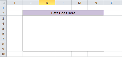
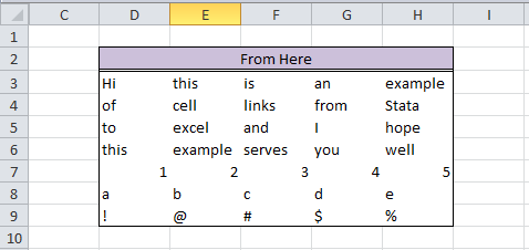
However, with a few simple Mata commands, the crisscross of equal signs, dollar signs, and formulas can turn a repetitive task into a few simple copy-and-paste commands. There is also less room for error. For fun, we'll do this entire thing in Mata. First, we need to decide how many observations/variables we need. Let’s look at our current workbook and target workbook.
So we need 5 columns and 7 rows, with columns from D to H and rows from 3 to 9 in our BookB set. Write it:
mata:
st_addobs(7)
st_addvar("str255", "v" :+ strofreal(1..5))
Starting with a blank dataset, add seven observations. From there, we create 5 variables (v1 v2 v3 v4 v5) that are all of type str255. This is a placeholder value for long equations. The second part of this command “v” :+ strofreal(1..5) is my favorite part about Mata. The colon operator (:+) is an element-wise operator that is super helpful. No more Matrix conformability errors (well maybe a few). It creates the matrix:
("v1", "v2", "v3", "v4", "v5")
without much work and allows for any number of variables! Sidenote – changing (1..5) to (1..500000) took about 3 seconds to create 500,000 v#’s. Next, let’s set up our workbook name: bookname = "'C:\Users\wmmatsuo\Desktop\[BookB.xlsx]Linked'!" Specify the location of the workbook with the file name in square brackets and enclose the sheet name in apostrophes. End that expression with an exclamation point! Since we know we want D through H, and cells 3-9, we can write the following: cols = numtobase26(4..8) rows = strofreal(3::9) numtobase26() turns 4 through 8 into D through H. For more information see my previous post on its inverse. The rows variable is a column vector containing values 3 through 9. Now it’s time to build our expression: expr = "=" :+ bookname :+ "$" :+ J(7, 1, cols) :+ "$" :+ rows We put an equals sign in front of everything so that Excel will know we’re calling an equation. Follow that with the workbook name. If you didn’t know, dollar signs in excel will lock your formulas so they don’t move when you copy formulas from one cell to another. We’ll put those in as well. The next part, J(7, 1, cols), takes our column letters and essentially repeats it seven rows down. Thanks to the colon operator, we just have to add another dollar sign to all elements of the matrix and our row numbers. Since the new cols matrix contains seven rows, and our row vector contains seven rows, it knows to repeat the row values for all columns. Let’s just put that matrix back into Stata and compress our variables.
st_sstore(., ("v" :+ strofreal(1..5)), expr)
stata("compress")
end
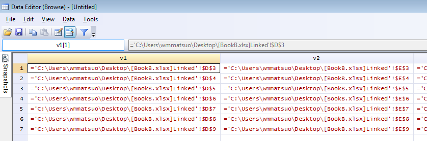
And voilà, we have a set of equations ready to copy into Excel. One quick tip: set your copy preferences so that when you copy the formulas, you won’t also copy variable names by going to edit->preferences->data editor-> uncheck “Include variable names on copy to clipboard”. Now just copy the equations directly from your Stata browse window into Excel, and enjoy those sweet results! 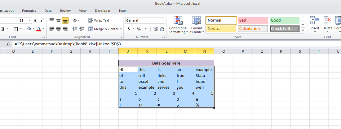
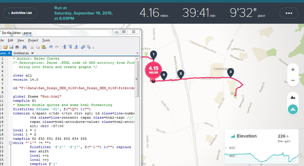
In other news, this post built upon the putexcel linking discoveries found over at belenchavez.com - who recently had her Fitbit stolen! Follow her journey to get it back on her website or on Twitter - hopefully she'll be able to coerce the thief into returning the device.
This post is one of my white whales – the problem that has eluded me for far too long and drove me to the edge of insanity. I’m talking about writing binary. Now, let me be clear when I say that I am far from a computer scientist: I don’t think in base 16, I don’t dream in assembly code, I don’t limit my outcomes to zeros and ones. I do, however, digest material before writing about it, seek creative and efficient solutions to problems, and do my best to share this information with others (that’s where you come in).
First, let’s create a fake dataset with help from Nick Cox’s egenmore ssc command:
set obs 300
forvalues i = 1/200 {
        gen x`i' = round(runiform()*50*_n)
}

gen id = _n
reshape long x, i(id) j(vars)
egen count = xtile(x), nq(30)
keep id vars count
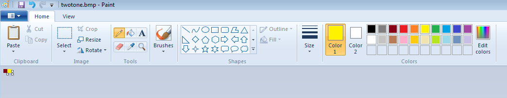
Today we will be making a bitmap of a map for Fitbit activities by writing bits of binned colors in a binary file. Alliteration aside, this post pulls from various sources and is intended to cover a great deal of topics that might be foreign to the average Stata user – in other words, hold on tight! It’s going to be a bumpy bitmap ride as we cover three major topics: (1) Color Theory, (2) Bitmap Structures, and (3) Writing Binary Files using Stata. Color Theory
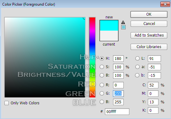
In creating gradients, it was recommended to me to use a Hue, Saturation, Value (HSV) linear interpolation rather than the Red, Green, Blue (RGB) interpolation because it looks more “natural.” I will not argue this point, as I know nothing about it. For me, I know that if I play with the sliders in Photoshop, it automatically changes the numbers and I never have to think about what it’s actually doing in the conversion. In order to convert from RGB to HSV and vice versa, I used the equations provided here – to learn about what’s going on, Wikipedia has a great article on the HSV cones!
|
|||||||||||

HSV Gradient with a 5 px Gaussian Blur
|

RGB Gradient with a 5 px Gaussian Blur
|
| bitmap.do |
I’m personally extremely excited to reveal this next set of blog posts because it ties together so many different concepts. This means that it will be broken out into several different parts. However, the complexity also comes at a cost. I thought I would be done by now – the struggle is real!
While I continue to do my research, I’ve added a quick snippet of what’s to be expected:

Author
Will Matsuoka is the creator of W=M/Stata - he likes creativity and simplicity, taking pictures of food, competition, and anything that can be analyzed.
For more information about this site, check out the teaser above!
Archives
July 2016
June 2016
March 2016
February 2016
January 2016
December 2015
November 2015
October 2015
September 2015
Categories
All
3ds Max
Adobe
API
Base16
Base2
Base64
Binary
Bitmap
Color
Crawldir
Email
Encryption
Excel
Exif
File
Fileread
Filewrite
Fitbit
Formulas
Gcmap
GIMP
GIS
Google
History
JavaScript
Location
Maps
Mata
Music
NFL
Numtobase26
Parsing
Pictures
Plugins
Privacy
Putexcel
Summary
Taylor Swift
Twitter
Vbscript
Work
Xlsx
XML
 RSS Feed